Microsoft Excel is a versatile and user-friendly application, most of the time, you find more than one solution to resolve a problem

In one of my post, I covered trick to convert cardinal number and date to ordinal (ordinal-number-and-ordinal-date-in-excel) with the help of formulas. You can achieve the same goal using conditional formatting, just follow the trick, I am going to cover in this post

Suppose, we have to convert cardinal number in the range “B2:B26” to ordinal number. To achieve the same, follow the instructions as explained below:

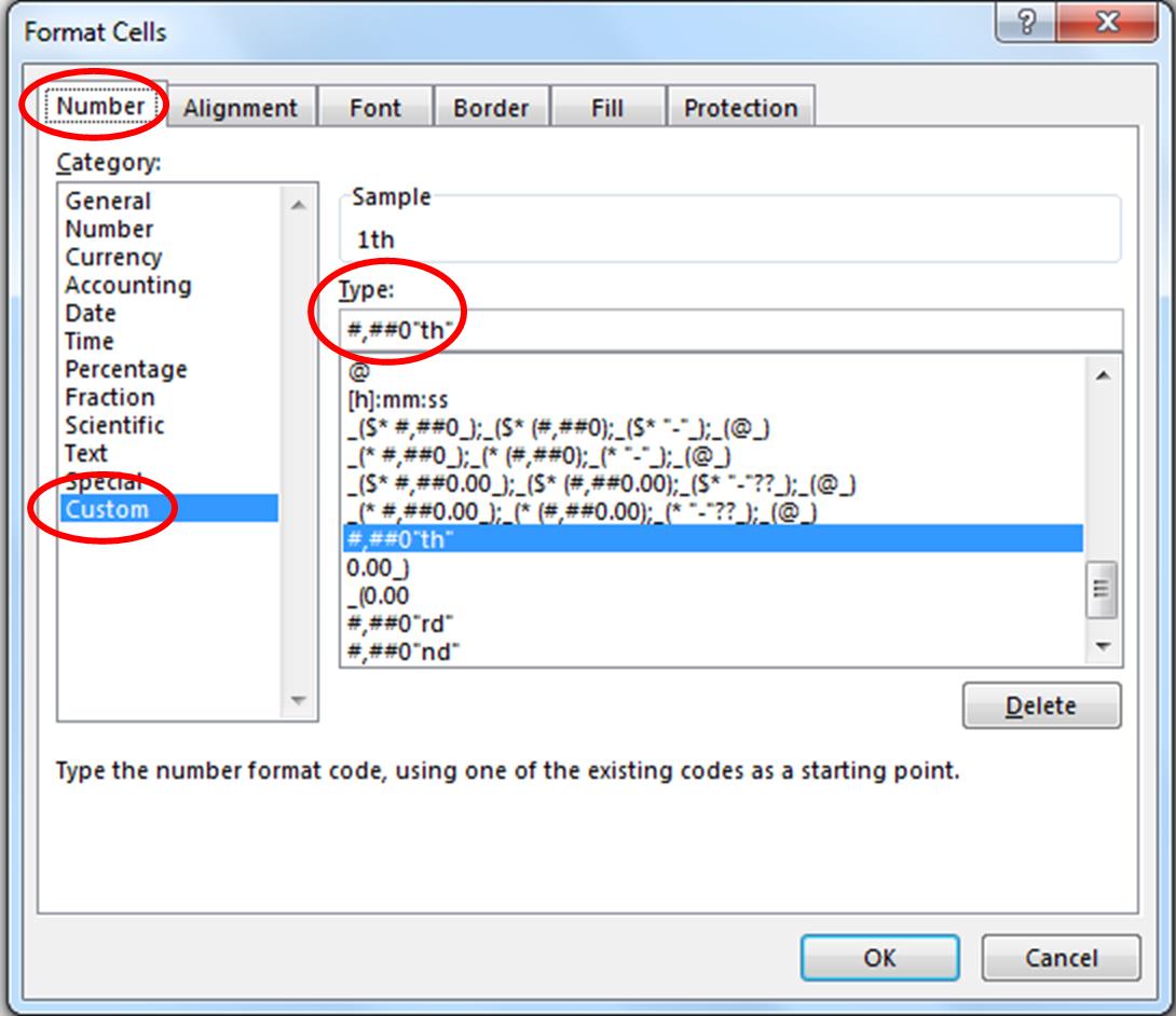
Select the range “B2:B26” and press Ctrl+1, a new pop-up window will open as shown hereunder:

From the window opened; select first tab viz. “Number”

Now, from Category list select the “Custom” and update the space below “Type” with #,##0″th” and press “OK” to close the window
With our above actions, we have changed the number format of the selected cells and have added suffix “th” to all the numbers in the selected range

To achieve the goal, we have to update three more conditions:

• If a number ends with “1”, but last two digits are not “11” add “st”
• If a number ends with “2”, but last two digits are not “12” add “nd”
• If a number ends with “3”, but last two digits are not “13” add “rdt”

For updating the first condition to correct the number ending with “1”, keep the required range selected and go to

HOME > Styles > Conditional Formatting > New Rule… > Use a formula to determine which cells to format

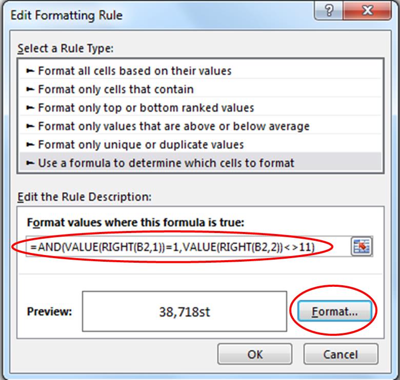
A pop-up window as shown below will appear:

Update the below formula as shown in the above picture

=AND(VALUE(RIGHT(B2,1))=1,VALUE(RIGHT(B2,2))<>11)

Now, click the “Format…” button (highlighted in the above picture)

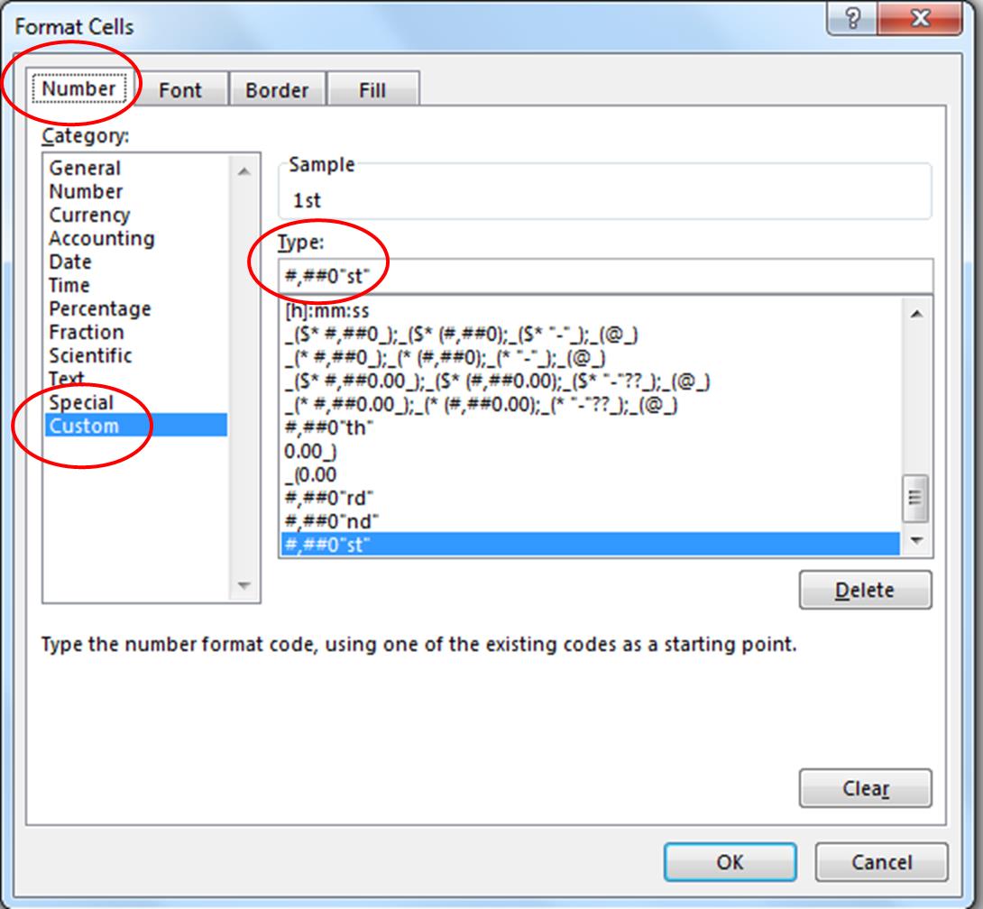
By clicking the “Format…” button, same “Format Cell” window will open (as appeared by pressing “Ctrl+1”). As done earlier, select the “Number” tab and “Custom” from the category list and this time update the space below “Type” with #,##0″st” as shown in below picture:

We have updated the first condition, but we have to repeat the above process to update the 2nd and 3rd formula and formatting conditions as explained above, for that again, go to:

HOME > Styles > Conditional Formatting > New Rule… > Use a formula to determine which cells to format

This time update the below formula to rectify the number that ends with 2:

=AND(VALUE(RIGHT(B2,1))=2,VALUE(RIGHT(B2,2))<>12)

Do remember to update formatting condition: #,##0″nd” in “Format Cells” window by clicking “Format…” button after updating the formula

Finally, repeat the process again to update the below formula to rectify the number ending with 3:

=AND(VALUE(RIGHT(B2,1))=3,VALUE(RIGHT(B2,2))<>13) ;

After updating the formula, update the condition #,##0″rd” as explained above

With this the numbers in the selected range will become ordinal numbers, now if you change the number in the range the suffix will change accordingly

To create ordinal number at any other range in same workbook or in any other workbook, just copy and paste any cell from the range, you applied above conditions. You are not required to update all the conditions again 

In case you have any query regarding above, you may send the same as comment to this blog