To generate Ordinal Number and Ordinal Date in excel.

An Ordinal Number is a number that tells the position of something in a list, such as 1st, 2nd, 3rd, 4th, 5th etc.

An Ordinal Date denotes the position of a day in a given month and year; e.g., 8th June, 2020

To achieve this we have to add a suffix after each number, based upon its value, in order to show its position; e.g., “st” with 1 makes it 1st. In case of date we have to check value of day which must be in between 1 to 31 and add suffix accordingly.

• If last one digit of number is 1, but last 2 digits are not equal to 11, add “st” as suffix
• If last one digit of number is 2, but last 2 digits are not equal to 12, add “nd” as suffix
• If last one digit of number is 3, but last 2 digits are not equal to 13, add “rd” as suffix
• In all other cases, add “th” as suffix

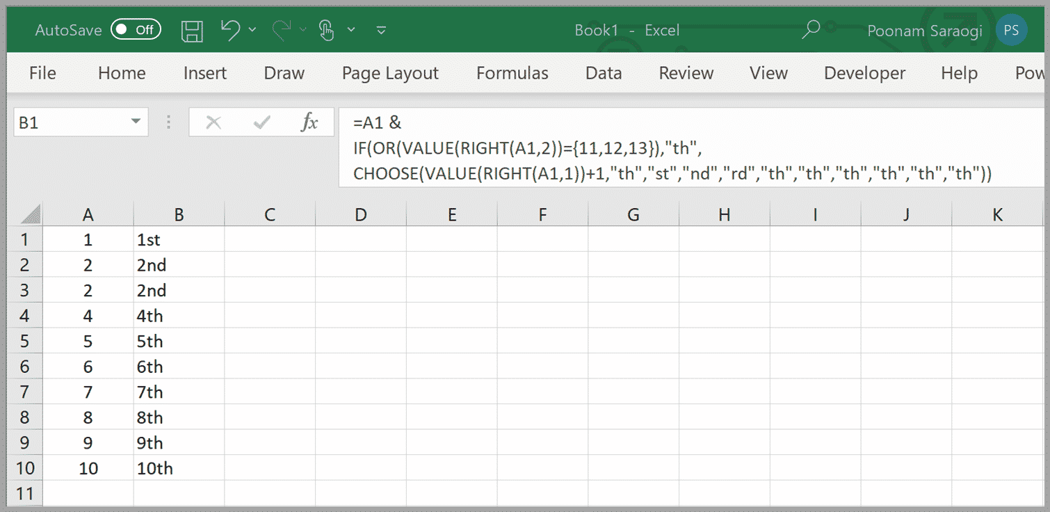
If number is in cell “A1” insert below formula in cell “B1” (“A1” and “B1” are used for example only, this’ll work in any 2 sets of cells)

=A1 &
IF(OR(VALUE(RIGHT(A1,2))={11,12,13}),”th”,
CHOOSE(VALUE(RIGHT(A1,1))+1,”th”,”st”,”nd”,”rd”,”th”,”th”,”th”,”th”,”th”,”th”))

In the 1st line of formula for Ordinal Numbers, we have taken number itself. In 2nd line we ensure that if last two digits of number are 11, 12 or 13 then add “th” as suffix. In last line we instruct excel to choose a value based on last digit of number. “CHOOSE” function will give error if last digit is “0”; hence added 1.

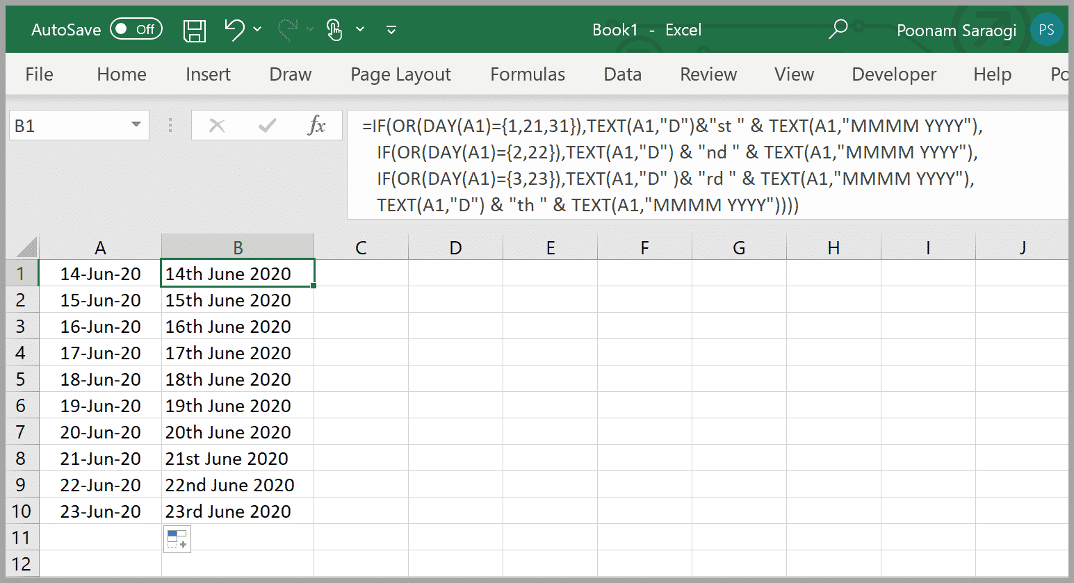
For date number formula will not work, use below formula in cell “B1” if date is in “A1” to convert date as “14th June, 2020” (“A1” and “B1” are used for example only, this’ll work in any 2 sets of cells).

=IF(OR(DAY(A1)={1,21,31}),TEXT(A1,”D”)&”st ” & TEXT(A1,”MMMM YYYY”),
IF(OR(DAY(A1)={2,22}),TEXT(A1,”D”) & “nd ” & TEXT(A1,”MMMM YYYY”),
IF(OR(DAY(A1)={3,23}),TEXT(A1,”D” )& “rd ” & TEXT(A1,”MMMM YYYY”),
TEXT(A1,”D”) & “th ” & TEXT(A1,”MMMM YYYY”))))

For Ordinal Date formula, we have to check numbers between 1 to 31 only, and we have used a different technique. In 1st line excel add “st” with day value if it’s 1, 21 or 31. In 2nd line suffix “nd” is added if day value is 2 or 22 and in 3rd line it add “rd” in case of 3 or 23. Finally add “th” for all other day values.

Once you add the suffix number will become text and you can’t use the same in calculation. In case you require to use the same use below formula to get number value from cell “A1”

=VALUE(LEFT(A1,LEN(A1)-2))