An excel worksheet is often used to update daily data. Suppose we enter per day sales by each engineer of the company in an excel worksheet. In such cases the number of rows is not fixed and extra rows are required to be added on daily basis. In turn you have to change your formula for total sales. One option is in your formula that you can cover entire column containing the sales data figures but I am not in favour of this because such formulas are error prone. If someone by mistake put the figures in this column our result will be wrong.

So, today our Goal is to create an auto extendable range in Excel, so that you don’t have to change your formula time and again as explained above

Solution to such problem is “Dynamic Named Range”, you can create a dynamic named range with excel’s built in function “OFFSET”. Syntax for “OFFSET” is as under:

OFFSET(reference, rows, cols, [height], [width])

In the above formula first three arguments are mandatory and last two are optional

In the first argument “reference” you have to insert the address of base cell, if this argument is missing you will get “#VALUE!” error.

By updating “rows” you can move up or down rows from the base cell, updated in “reference”, if the value is +ve you will move down and to move upward from the base cell use –ve sign. Similarly with +ve value in “cols”, you can move to columns in right of the base cell and to left if the value is –ve. If sufficient number of rows or columns are not available as per value of “rows” or “cols” you will get “#REF!” error

You can select specific number of rows or columns by updating “height” and “width” respectively. Value for the arguments must be +ve.

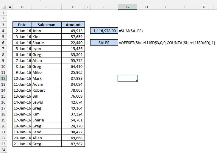
Suppose your data is in column “D” starting from fourth row and third row containing the header for your data in “Sheet1”. To create the dynamic named range follow the following steps:

• In “Formulas” tab click “Name Manager” from “Defined Names” group.
• A pop-up window will open; click “New” from this.
• A new window for creating new name will open.
• Enter the name for your dynamic range e.g. “SALES”.
• Define scope of named range, by default Excel will select “Workbook”
• In refers to put the below formula

=OFFSET(Sheet1!$D$3,0,0,COUNTA(Sheet1!$D:$D),1)

With this excel has created dynamic named range “SALES” for you. You can use this named range in your formula like

=SUM(SALES)

This formula will always show the correct figure of sales. If you add or delete some sales figures dynamic range will be adjusted accordingly and the formula will show correct amount.

For the first argument, we have updated “Sheet1!$D$3” as address of base cell, in this case header cell of our data. No change with second and third arguments as both the values are “0”. For “height” argument, we have used formula “COUNTA(Sheet1!$D:$D)”, this formula count the filled cells in column “D” (whenever you update data in cells, the value of height will increase) and pass the argument to “OFFSET” function which in turn select all filled cells for calculation. Finally, we have updated “width” as “1” to ensure “OFFSET” select cells of one column only

Please ensure that there is no blank cell in between else the formula will not show the correct figure.