Today our goal is to calculate EMI (Equated Monthly Installment) with change of interest rate and loan amount

Home loans in most countries are available at flexible interest rates. It means your interest rates may go down or up, based upon the market conditions. In such a scenario, you must strive to know how your EMI (payment for the loan) for a period will change, with a change in the interest rate

A number of financial functions are available in Excel. To calculate the EMI, we can use function “PMT”. Syntax for “PMT” is as under:

PMT(rate, nper, pv, [fv], [type])

In the above function first three arguments are mandatory and last two are optional. For first argument “rate” we have to update monthly rate of interest for the loan, for “nper” number of payments of loan, for “pv” present value or amount of loan taken, for “fv” future value or balance after last payment (it’s assumed to be “0”), and finally for “type” put “0” if payment is due at the end of the period and “1” if it’s due at the beginning. Default value for “type” is also “0”

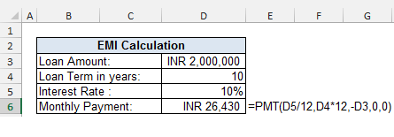
Suppose we have to calculate EMI on loan of 2 Million (20 lacs) Indian rupees for 10 years at the interest rate of 10% p.a.

Here, “rate” is converted to monthly basis by dividing with 12 (months); i.e., “10%/12”, “nper” will be “10*12” i.e. 120 (number of EMIs), value of “pv” or loan amount is 2,000,000, “fv” and “type” are equal to 0.

We can put the values directly in formula as shown here below:

=PMT(10%/12,10*12,2000000,0,0)

You may put the values in cells also and can use the cell addresses in formula as under:

Please note that in the above formula, I have used –ve sign before loan amount, if you don’t use it you will get your answer in –ve. Also in default setting result will be shown in currency format, which you may change as required.

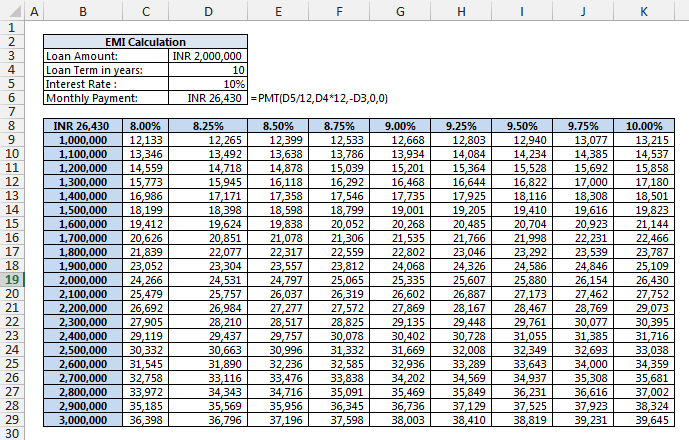
Now, I will explain how to create a “Data Table” for different loan amount or principal at different interest rates, one of the most under-utilized feature of excel. To create “Data Table” follow the following instructions.

Calculate the EMI amount with PMT function, this we have already done in the example above. It doesn’t matter what you select as loan amount and interest rate but select period (in this case it is 10 years) for which you want to generate the “Data Table” as shown in the example picture above in cells B2:D6.

Insert different rates of interest in cells from C8 to S8 and different loan amounts in cells range B9:B29. (Remember that No. of years are fixed at 10 years)

In cell B8 insert the formula “=D6”.

Now, select the range B8:S29 and choose Data►Data Tools►What-If Analysis►Data Table, a new pop-up window will open

In “Data Table” window insert D5 (Rate of interest) in Row input cell, and D3 (Loan or principal) in Column input cell, you may input the cell value by selecting the cells also.
Now, press OK so that excel can update your table with required data in lightning speed.

Your “Data Table” will be ready as shown below.

In case, you need to check the data for some other number of years (5 years or 12 years or 20 years), you need to simply update the cell “D4” with required number of years, and the table will get updated automatically